sphinx_ipypublish_all.ext3. Writing Markdown
In IPyPublish, all Markdown content is converted via
Pandoc. Pandoc
alllows for filters to be applied
to the intermediary representation of the content, which IPyPublish
supplies through a group of
panflute filters, wrapped
in a single ‘master’ filter; ipubpandoc. This filter extends the
common markdown syntax to:
Correctly translate pieces of documentation written in other formats (such as using LaTeX commands like
\citeor RST roles like:cite:)Handle labelling and referencing of figures, tables and equations, and add additional formatting options.
ipubpandoc is detached from the rest of the notebook conversion
process, and so can be used as a standalone process on any markdown
content:
$ pandoc -f markdown -t html --filter ipubpandoc path/to/file.md
See also
The PDF representation of this notebook
Adding a stylesheet to slides, for the notebook document level metadata options.
3.1. Converting Notebooks to RMarkdown
RMarkdown is a plain text representation of the workbook. Thanks to jupytext, we can easily convert an existing notebooks to RMarkdown (and back):
$ jupytext --to rmarkdown notebook.ipynb
$ jupytext --to notebook notebook.Rmd            # overwrite notebook.ipynb (remove outputs)
$ jupytext --to notebook --update notebook.Rmd   # update notebook.ipynb (preserve outputs)
Alternatively, simply create a notebook.Rmd, and add this to the top of the file:
---
jupyter:
  ipub:
    pandoc:
      convert_raw: true
      hide_raw: false
      at_notation: true
      use_numref: true
  jupytext:
    metadata_filter:
      notebook: ipub
    text_representation:
      extension: .Rmd
      format_name: rmarkdown
      format_version: '1.0'
      jupytext_version: 0.8.6
  kernelspec:
    display_name: Python 3
    language: python
    name: python3
---
Important
To preserve ipypublish notebook metadata, you must
add:
{"jupytext": {"metadata_filter": {"notebook": "ipub"}}}
to
your notebooks metadata before conversion.
Note
If a file with a .Rmd extension is supplied to
nbpublish, it
will automatically call jupytext and convert it.
So it is possible
to only ever write in the RMarkdown format!
3.2. Working with RMarkdown files
The recommended way to edit RMarkdown files is in Visual Studio Code, with the Markdown Preview Enhanced extension. Add this to your VS Code Settings:
{
    "files.associations": {
        "*.Rmd": "markdown"
    },
    "markdown-preview-enhanced.usePandocParser": true,
    "markdown-preview-enhanced.pandocArguments": "--filter=ipubpandoc",
    "markdown-preview-enhanced.enableScriptExecution": true
}
If you are using a Conda environment, you may also need to use:
{
    "markdown-preview-enhanced.pandocPath": "/anaconda/envs/myenv/bin/pandoc",
    "markdown-preview-enhanced.pandocArguments": "--filter=/anaconda/myenv/lsr/bin/ipubpandoc"
}
You will now be able to open a dynamic preview of your notebook, with executable code cells:
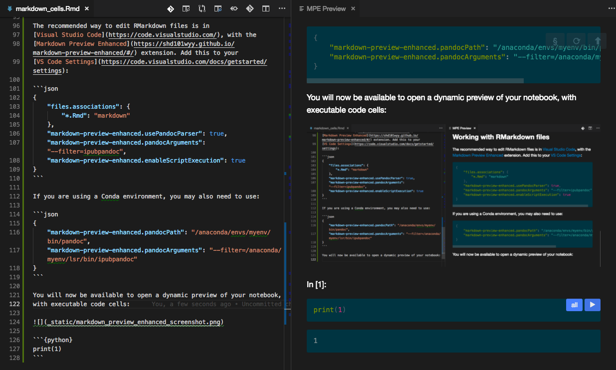
Fig. 3.2.1 MPE Screenshot
[1]:
print(1)
1
See also
VS Code Extensions: Markdown Extended and markdownlint
3.3. Inter-Format Translation
ipubpandoc attempts to detect any segments of documentation written
in LaTeX or Sphinx
reStructuredText
(and HTML citations), and convert them into a relevant panflute
element.
Because of this we can write something like this:
- citations in @ notation [@zelenyak_molecular_2016; @kirkeminde_thermodynamic_2012]
- citations in rst notation :cite:`zelenyak_molecular_2016,kirkeminde_thermodynamic_2012`
- citations in latex notation \cite{zelenyak_molecular_2016,kirkeminde_thermodynamic_2012}
- citation in html notation <cite data-cite="kirkeminde_thermodynamic_2012">text</cite>

$$a = b + c$$ {#eqnlabel}

- a reference in @ notation =@eqnlabel {.capital}
- a reference in rst notation :eq:`eqnlabel`
- a reference in latex notation \eqref{eqnlabel}

.. note::

    a reference in latex notation within an RST directive \eqref{eqnlabel}
and it will be correctly resolved in the output document:
citation in html notation [KR12]
a reference in @ notation Eq. 3.3.1
a reference in rst notation Eq. 3.3.1
a reference in latex notation Eq. 3.3.1
Note
a reference in latex notation within an RST directive Eq. 3.3.1
Inter-format translation is turned on by default, but if you wish to turn it off, or hide it, simply add to the document metadata:
jupyter:
  ipub:
    pandoc:
      convert_raw: true
      hide_raw: false
3.4. Labelling, Formatting and Referencing Figures, Tables and Equations
ipubpandoc allows for figures, tables, equations and references to
be supplied with an ‘attribute container’. This is a braced section to
the side of the figures, equations, reference or table caption, that
parses on additional information to the formatter,
e.g. {#id .class-name attribute1=10}.
Attribute containers are turned on by default, but if you wish to turn them off, simply add to the document metadata:
jupyter:
  ipub:
    pandoc:
      at_notation: false
Tip
Zero or more Space is generally allowed between the element and the attribute container.
3.4.1. Figures
Figures can have an identifier and a width or height. Additionally,
placement will be used by LaTeX output.
{#fig:example width=50% placement='H'}
@fig:example

Fig. 3.4.1 Image caption
3.4.2. Tables
Tables can have an identifier and relative widths (per column).
Additionally, align will be used by LaTeX and HTML to set the
alignment of the columns (l=left, r=right, c=center)
Column 1 |
Column 2 |
|---|---|
1 |
2 |
3.4.3. Equations
Equations can have an identifier and an env denoting the amsmath
environment.
$$2x &= 8 \\ 3x + 9y &= -12$$ {#eqn:example2 env=align}
Note
Labelled math must be ‘display math’, rather than inline, i.e. wrapped in double dollars.
3.4.4. References
Pandoc references are denoted by @, with an optional prefix, and
multiple references can be wrapped in square brackets:
Citation [@zelenyak_molecular_2016; @kirkeminde_thermodynamic_2012]

Glossary Terms: %@gtkey2, &@akey2, &@symbol2
Glossary Terms: Name, MA, \(\pi\)
Note
Citations in sphinx are provided by the excellent sphinxcontrib-bibtex extension, and glossary referencing is provided by the equally good ipypublish.sphinx.gls
References can have attributes; latex (defining the LaTeX tag to
use), rst (defining the RST role to use) and class .capital
(defining if HTML naming is capitalized)
@fig:example {.capital latex=cref rst=numref}, [@eqnlabel;@eqn:example2] {latex=eqref rst=eq}
Fig. 3.4.1, Eq. 3.3.1 and Eq. 3.4.1
A number of prefixes are available, as shorthand’s to define attributes:
prefix |
attribute |
|---|---|
“” |
{latex=cite rst=cite} |
“+” |
{latex=cref rst=numref} |
“!” |
{latex=ref rst=ref} |
“=” |
{latex=eqref rst=eq} |
“?” |
{.capital latex=Cref rst=numref} |
“&” |
{latex=gls rst=gls} |
“%” |
{.capital latex=Gls rst=glsc} |
?@fig:example, =[@eqnlabel;@eqn:example2]
Fig. 3.4.1, Eq. 3.3.1 and Eq. 3.4.1
Tip
Pandoc interprets (@label) as a numbered
example, so
instead use (@label{})
3.5. A Note on Implementation
To assign attributes to items, we use a preparation filter, to extract prefixes and attributes, and wrap the items in a Span containing them. For example:
$$a=1$$ {#a env=align}
will be transformed to:
<p>
<span id="a" class="labelled-Math" data-env="align">
<br />
<span class="math display">
<em>a</em> = 1
</span>
<br />
</span>
</p>
and
"+@label{ .class a=1} xyz *@label2* @label3{ .b}"
will be transformed to:
<p>
<span class="attribute-Cite class"
data-latex="cref" data-rst="numref" data-a="1">
<span class="citation" data-cites="label">
@label
</span></span>
xyz
<em><span class="citation" data-cites="label2">
@label2
</span></em>
<span class="attribute-Cite b">
<span class="citation" data-cites="label3">
@label3
</span></span>
</p>
Formatter filters, then look for these parent spans, to provide identifiers, classes and attributes.
Glossary
Bibliography
- KR12(1,2,3,4,5)
Alec Kirkeminde and Shenqiang Ren. Thermodynamic control of iron pyrite nanocrystal synthesis with high photoactivity and stability. Journal of Materials Chemistry A, 1(1):49–54, 2012. doi:10.1039/C2TA00498D.
- ZKT+16(1,2,3,4)
T. Yu Zelenyak, Kh T. Kholmurodov, A. R. Tameev, A. V. Vannikov, and P. P. Gladyshev. Molecular dynamics study of perovskite structures with modified interatomic interaction potentials. High Energy Chemistry, 50(5):400–405, 2016. doi:10.1134/S0018143916050209.